%matplotlib inline
import matplotlib.pyplot as plt
import matplotlib.tri as tri
import numpy as np
import adios as ad
plt.rcParams['figure.figsize'] = (6, 4)
cm = plt.cm.jet
subdir = 'totalf_itg_tiny/'
XGC mesh structure
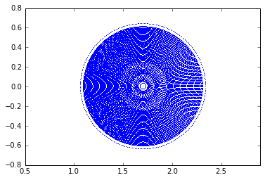
XGC mesh file (xgc.mesh.bp) contains the following variables: * n_n: the number of nodes * n_t: the number of cells * rz: node coodinates (shape: {n_n, 2}) * nd_connect_list: connection list or cell definition (shape: {n_t, 3})
with ad.file(subdir + 'xgc.mesh.bp') as f:
    nnodes = f['n_n'][...]
    ncells = f['n_t'][...]
    rz = f['rz'][...]
    conn = f['nd_connect_list'][...]

R = rz[:,0]
Z = rz[:,1]
plt.plot(R, Z, ',');
plt.axis('equal');
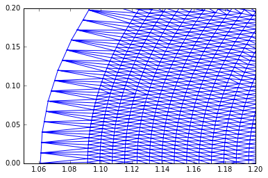
If we zoom, we can see the unstructued mesh clearly:
trimesh = tri.Triangulation(R, Z, conn)
plt.triplot(trimesh);
plt.xlim([1.05, 1.2])
plt.ylim([0.0, 0.2]);
XGC field data
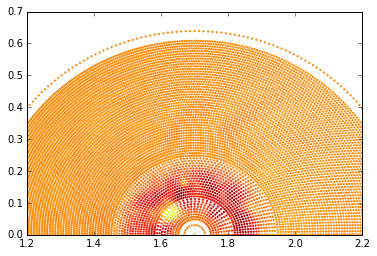
Let’s draw one of XGC field data: dpot in xgc.3d.xxxxx.bp.
The shape of dpot is (n_n, nphi) where n_n is the number of grid nondes and nphi is the number of planes used in XGC simulation.
with ad.file(subdir + 'xgc.3d.08800.bp') as f:
    dpot = f['dpot'][...,0]
plt.scatter(R, Z, c=dpot, marker='.', lw = 0);
plt.xlim([1.2, 2.2])
plt.ylim([0.0, 0.7]);
trimesh = tri.Triangulation(R, Z, conn)
plt.tricontourf(trimesh, dpot, cmap=cm);
plt.axis('equal');
plt.colorbar();
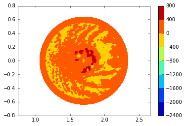
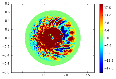
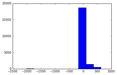
Let’s refine the plot by restricting the dpot range to see more turbulent behavior.
plt.hist(dpot);
def plot_dpot(dpot, levels=np.linspace(-20, 20, num=101), title=''):
    dp = dpot.copy()
    dp[dpot >= levels[-1]] = levels[-2]
    dp[dpot <= levels[0]] = levels[0]
    plt.tricontourf(trimesh, dp, levels, cmap=cm);
    plt.axis('equal');
    plt.colorbar();
    plt.title(title)
plot_dpot(dpot)
